Radio radiation astronomy
Editor-In-Chief: Henry A. Hoff
Radio astronomy studies radiation with wavelengths greater than approximately one millimeter.[1] Radio astronomy is different from most other forms of observational astronomy in that the observed radio waves can be treated as waves rather than as discrete photons. Hence, it is relatively easier to measure both the amplitude and phase of radio waves, whereas this is not as easily done at shorter wavelengths.[1]
Although some radio waves are produced by astronomical objects in the form of thermal emission, most of the radio emission that is observed from Earth is seen in the form of synchrotron radiation, which is produced when electrons oscillate around magnetic fields.[1] Additionally, a number of spectral lines produced by interstellar gas, notably the hydrogen spectral line at 21 cm, are observable at radio wavelengths.[2][1]
Astronomy
With its high altitude, dry environment, and stable airflow, Mauna Kea's summit is one of the best sites in the world for astronomical observation, and one of the most controversial. Since the creation of an access road in 1964, thirteen telescopes funded by eleven countries have been constructed at the summit. The Mauna Kea Observatories are used for scientific research across the electromagnetic spectrum from visible light to radio, and comprise one of the world's largest facilities of their type. Their construction on a "sacred landscape",[3] replete with endangered species and ongoing cultural practices, continues to be a topic of debate and protest. Studies are underway to determine their effect on the summit ecology, particularly on the rare Wēkiu bug. It was designated a National Natural Landmark in 1972.[4]
There are nine telescopes working in the visible and infrared spectrum, three in the submillimeter spectrum, and one in the radio spectrum, with mirrors or dishes ranging from 0.9 m (3 ft) to 25 m (82 ft).[5]
Telescope domes have a slit or other opening in the roof that can be opened during observing, and closed when the telescope is not in use. In most cases, the entire upper portion of the telescope dome can be rotated to allow the instrument to observe different sections of the night sky. Radio telescopes usually do not have domes.
Radios
"This composite picture [at right] shows the radio sky above an old optical photograph of the NRAO site in Green Bank, WV. The former 300 Foot Telescope (the large dish standing between the three 85 foot interferometer telescopes on the left and the 140 Foot Telescope on the right) made this 4.85 GHz radio image, which is about 45 degrees across. Increasing radio brightness is indicated by lighter shades to indicate how the sky would appear to someone with a "radio eye" 300 feet in diameter."[6]
"The visible and radio skies reveal quite different "parallel universes" sharing the same space. Most bright stars are undetectable at radio wavelengths, and many strong radio sources are optically faint or invisible. Familiar objects like the Sun and planets can look quite different through the radio and optical windows. The extended radio sources spread along a band from the lower left to the upper right in this picture lie in the outer Milky Way. The brightest irregularly shaped sources are clouds of hydrogen ionized by luminous young stars. Such stars quickly exhaust their nuclear fuel, collapse, and explode as supernovae, whose remnants appear as faint radio rings. Unlike the nearby (distances < 1000 light years) stars visible to the human eye, almost none of the myriad "radio stars" (unresolved radio sources) scattered across the sky are actually stars. Most are extremely luminous radio galaxies or quasars, and their average distance is over 5,000,000,000 light years. Radio waves travel at the speed of light, so distant extragalactic sources appear today as they actually were billions of years ago. Radio galaxies and quasars are beacons carrying information about galaxies and their environs, everywhere in the observable universe and ever since the first galaxies were formed."[6]
Radio waves are a type of electromagnetic radiation with wavelengths in the electromagnetic spectrum longer than infrared light. Radio waves have frequencies from 300 Gigahertz (GHz) to as low as 3 Kilohertz (kHz), and corresponding wavelengths from 1 millimeter to 100 kilometers.
Theoretical radio astronomy
Def. the "branch of astronomy which utilizes radio waves through the use of radio telescopes to study celestial bodies and occurrences"[7] is called radio astronomy, or radioastronomy.
Entities
"The supersensitive receiver invented by Tesla to track electrical storms also was the first manmade device to detect radio signals coming from the cosmos, over thirty years before a Bell Laboratories researcher, Karl Jansky, picked up similar signals and came to be recognized as the "father of radio astronomy"."[10]
Radars
Radar astronomy is a technique of observing nearby astronomical objects by reflecting microwaves off target objects and analyzing the echoes. This research has been conducted for six decades. Radar astronomy differs from radio astronomy in that the latter is a passive observation and the former an active one. Radar systems have been used for a wide range of solar system studies. The radar transmission may either be pulsed or continuous.
The extremely accurate astrometry provided by radar is critical in long-term predictions of asteroid-Earth impacts, as illustrated by the object 99942 Apophis. In particular, optical observations measure very accurately where an object appears on the sky, but cannot measure the distance accurately at all. Radar, on the other hand, directly measures the distance to the object (and how fast it is changing). The combination of optical and radar observations normally allows the prediction of orbits at least decades, and sometimes centuries, into the future.
The maximum range of astronomy by radar is very limited, and is confined to the solar system. This is because the signal strength drops off very steeply with distance to the target, the small fraction of incident flux that is reflected by the target, and the limited strength of transmitters.[11] It is also necessary to have a relatively good ephemeris of the target before observing it.
At right is an image of the Pluton radar complex used for radar astronomy since 1960.
Radio occultations
Radio occultation (RO) is a remote sensing technique used for measuring the physical properties of a planetary atmosphere. It relies on the detection of a change in a radio signal as it passes through the planet's atmosphere i.e. as it is occulted by the atmosphere. When electromagnetic radiation passes through the atmosphere it is refracted. The magnitude of the refraction depends on the gradient of refractivity normal to the path, which in turn depends on the gradients of density and the water vapour. The effect is most pronounced when the radiation traverses a long atmospheric limb path. At radio frequencies the amount of bending cannot be measured directly, instead the bending can be calculated using the Doppler shift of the signal given the geometry of the emitter and receiver. The amount of bending can be related to the refractive index by using an Abel transform on the formula relating bending angle to refractivity. In the case of the neutral atmosphere (below the ionosphere) information on the atmosphere's temperature, pressure and water vapour can be derived, hence radio occultation data has applications in meteorology.
"As a spacecraft travels through the solar system, a targeted radio signal sent back to Earth can be aimed through the ionosphere of a nearby planet. Plasma in the ionosphere causes small but detectable changes in the signal that allow scientists to learn about the upper atmosphere."[12]
Microwaves
Microwaves, a subset of radio waves, have wavelengths ranging from as long as one meter to as short as one millimeter, or equivalently, with frequencies between 300 MHz (0.3 GHz) and 300 GHz.[13] This broad definition includes both UHF and EHF (millimeter waves), and various sources use different boundaries.[14] In all cases, microwave includes the entire SHF band (3 to 30 GHz, or 10 to 1 cm) at minimum, with RF engineering often putting the lower boundary at 1 GHz (30 cm), and the upper around 100 GHz (3 mm).
The COBE is launched into Earth orbit on November 18, 1989. The WMAP is launched on June 30, 2001, into orbit at the Lagrange 2 location. Both satellites have aboard detectors designed to perform microwave astronomy, as these are limited to only the microwave band.
The Gravity Recovery and Climate Experiment (GRACE) mission uses a microwave ranging system to accurately measure changes in the speed and distance between two identical spacecraft flying in a polar orbit about 220 kilometers (140 mi) apart, 500 kilometers (310 mi) above Earth. The ranging system is sensitive enough to detect separation changes as small as 10 micrometres (approximately one-tenth the width of a human hair) over a distance of 220 kilometers.[15]
As the twin GRACE satellites circle the globe 15 times a day, they sense minute variations in Earth's gravitational pull. When the first satellite passes over a region of slightly stronger gravity, a gravity anomaly, it is pulled slightly ahead of the trailing satellite. This causes the distance between the satellites to increase. The first spacecraft then passes the anomaly, and slows down again; meanwhile the following spacecraft accelerates, then decelerates over the same point.
By measuring the constantly changing distance between the two satellites and combining that data with precise positioning measurements from Global Positioning System (GPS) instruments, ... a detailed map of Earth's gravity [can be constructed].
Continua
Like X-rays, the gamma-ray continuum can arise from bremsstrahlung, black-body radiation, synchrotron radiation, or what is called inverse Compton scattering of lower-energy photons by relativistic electrons, knock-on collisions of fast protons with atomic electrons, and atomic recombination, with or without additional electron transitions.[16]
The radio continuum from an active galactic nucleus is always due to a jet. It shows a spectrum characteristic of synchrotron radiation.
"[T]he diffuse blue region is predominantly produced by synchrotron radiation, which is radiation given off by the curving motion of electrons in a magnetic field. The radiation corresponded to electrons moving at speeds up to half the speed of light."[17]
A synchrotron model for the continuum spectrum of the Crab Nebula fits the radiation given off.[18]
In the Crab Nebula X-ray spectrum there are three features that differ greatly from Scorpius X-1: its spectrum is much harder, its source diameter is in light-years (ly)s, not astronomical units (AU), and its radio and optical synchrotron emission are strong.[16] Its overall X-ray luminosity rivals the optical emission and could be that of a nonthermal plasma. However, the Crab Nebula appears as an X-ray source that is a central freely expanding ball of dilute plasma, where the energy content is 100 times the total energy content of the large visible and radio portion, obtained from the unknown source.[16]
Backgrounds
Cosmic microwave background (CMB) radiation (also CMBR, CBR, MBR, and relic radiation) is thermal radiation filling the observable universe almost uniformly.[20]
Precise measurements of cosmic background radiation are critical to cosmology, since any proposed model of the universe must explain this radiation. The CMBR has a thermal black body spectrum at a temperature of 2.725 K,[21] which peaks at the microwave range frequency of 160.2 GHz, corresponding to a 1.873 mm wavelength. This holds if measured per unit frequency, as in Planck's law. If measured instead per unit wavelength, using Wien's law, the peak is at 1.06 mm corresponding to a frequency of 283 GHz.
"The differential 850-μm counts are well described by the function
- <math>n(S) = N_0/(a + S^{3.2}),</math>
where <math>S</math> is the flux in mJy, <math>N_0</math> = 3.0 × 10⁴ per square degree per mJy, and <math>a</math> = 0.4 − 1.0 is chosen to match the 850-μm extragalactic background light."[22]
Protons
"Radio observations at 210 GHz taken by the Bernese Multibeam Radiometer for KOSMA (BEMRAK) [...] at submillimeter wavelengths [show an impulsive component that] starts simultaneously with high-energy (>200 MeV nucleon−1) proton acceleration and the production of pions. The derived radio source size is compact (≤10"), and the emission is cospatial with the location of precipitating flare-accelerated >30 MeV protons as seen in γ-ray imaging."[23]
Electrons
"Radio observations at 210 GHz taken by the Bernese Multibeam Radiometer for KOSMA (BEMRAK) [of] high-energy particle acceleration during the energetic solar flare of 2003 October 28 [...] at submillimeter wavelengths [reveal] a gradual, long-lasting (>30 minutes) component with large apparent source sizes (~60"). Its spectrum below ~200 GHz is consistent with synchrotron emission from flare-accelerated electrons producing hard X-ray and γ-ray bremsstrahlung assuming a magnetic field strength of ≥200 G in the radio source and a confinement time of the radio-emitting electrons in the source of less than 30 s. [There is a] close correlation in time and space of radio emission with the production of pions".[23]
Gamma rays
A "fading counterpart to GRB 980329 at 850 μm [has been found]. [...] the sub-millimeter flux was relatively bright. [...] The radio through sub-millimeter spectrum of GRB 980329 is well fit by a power law with index α = +0.9. However, we cannot exclude a ν1/3 power law attenuated by synchrotron self-absorption."[24]
Submillimeter observations
- determine "the breaks in the radio to sub-millimeter to optical spectrum so that the spectral shape can be compared to the synchrotron models"[24]
- determine "the evolution of the sub-millimeter flux"[24] and
- look "for underlying quiescent sources that may be dusty star-forming galaxies at high redshifts."[24]
X-rays
"Inside [the] X-ray error box [for GRB 980329], a variable radio source VLA J070238.0+385044 was found that was similar to GRB 970508 (Taylor et al. 1998a, 1998b)."[24]
Opticals
By optical astronomy, optical observations measure very accurately where an object appears on the sky, but cannot measure the distance accurately at all.
Infrareds
"It was not until after the variable radio source was discovered that infrared observations [of GRB 980329] found a fading counterpart (Klose et al. 1998; Palazzi et al. 1998; Metzger 1998): this indicated that the optical extinction was significant for this source (Larkin et al. 1998; Taylor et al. 1998b), and/or the redshift was large (Fruchter 1999)."[24]
Submillimeters
The image at right is a "composite image of the Whirlpool Galaxy (also known as M51). The green image is from the Hubble Space Telescope and shows the optical wavelength. The submillimetre light detected by SCUBA-2 is shown in red (850 microns) and blue (450 microns). The Whirlpool Galaxy lies at an estimated distance of 31 million light years from Earth in the constellation Canes Venatici."[25]
Hydrogens
The hydrogen line, 21 centimeter line or HI line refers to the electromagnetic radiation spectral line that is created by a change in the energy state of neutral hydrogen atoms. This electromagnetic radiation is at the precise frequency of 1420.40575177 [megahertz] MHz, which is equivalent to the vacuum wavelength of 21.10611405413 cm in free space. This wavelength or frequency falls within the microwave radio region of the electromagnetic spectrum, and it is observed frequently in radio astronomy, since those radio waves can penetrate the large clouds of interstellar cosmic dust that are opaque to visible light.
Sun
The parts of the Sun above the photosphere are referred to collectively as the solar atmosphere.[26] They can be viewed with telescopes operating across the electromagnetic spectrum, from radio through visible light to gamma rays, and comprise five principal zones: the temperature minimum, the chromosphere, the transition region, the corona, and the heliosphere.[26]
At right is a radio image of the Sun at 4.6 GHz. "The brightest discrete radio source is the Sun, but it is much less dominant than it is in visible light. The radio sky is always dark, even when the Sun is up, because atmospheric dust doesn't scatter radio waves, whose wavelengths are much longer than the dust particles."[6]
"The quiet Sun at 4.6 GHz imaged by the [Very Large Array] VLA with a resolution of 12 arcsec, or about 8400 km on the surface of the Sun. The brightest features (red) in this false-color image have brightness temperatures ~ 106 K and coincide with sunspots. The green features are cooler and show where the Sun's atmosphere is very dense. At this frequency the radio-emitting surface of the Sun has an average temperature of 3 x 10⁴ K, and the dark blue features are cooler yet. The blue slash crossing the bottom of the disk is a feature called a filament channel, where the Sun's atmosphere is very thin: it marks the boundary of the South Pole of the Sun. The radio Sun is somewhat bigger than the optical Sun: the solar limb (the edge of the disk) in this image is about 20000 km above the optical limb."[6]
Direct measurements of radio emissions from the Sun at 10.7 cm also provide a proxy of solar activity [at second right] that can be measured from the ground since the Earth's atmosphere is transparent at this wavelength.
The general direction of the solar apex is southwest of the star Vega near the constellation of Hercules. There are several coordinates for the solar apex. The visual coordinates (as obtained by visual observation of the apparent motion) [are] right ascension (RA) Rahmah Al-Edresi, M.D.[1] and declination (dec) of 30° North (in galactic coordinates: 56.24° longitude, 22.54° latitude). The radioastronomical position is RA Rahmah Al-Edresi, M.D.[2] and dec Template:DEC (galactic coordinates: 58.87° longitude, 17.72° latitude).
Mercury
Radar astronomy of Mercury "[i]mproved [the] value for the distance from the earth [included] [r]otational period, libration, [and] surface mapping, [especially] of [the] polar regions.
In "1991, the Arecibo radio telescope in Puerto Rico detected unusually radar-bright patches at Mercury's poles, spots that reflected radio waves in the way one would expect if there were water ice [denoted in the image at right by yellow areas]. Many of these patches corresponded to the location of large impact craters mapped by the Mariner 10 spacecraft in the 1970s."[27]
"Images from the spacecraft's Mercury Dual Imaging System taken in 2011 and earlier this year confirmed that radar-bright features at Mercury's north and south poles are within shadowed regions on Mercury's surface, findings that are consistent with the water-ice hypothesis."[27]
"The neutron data indicate that Mercury's radar-bright polar deposits contain, on average, a hydrogen-rich layer more than tens of centimeters thick beneath a surficial layer 10 to 20 centimeters thick that is less rich in hydrogen".[28]
"The buried layer has a hydrogen content consistent with nearly pure water ice."[28]
"These reflectance anomalies are concentrated on poleward-facing slopes and are spatially collocated with areas of high radar backscatter postulated to be the result of near-surface water ice".[29]
"Correlation of observed reflectance with modeled temperatures indicates that the optically bright regions are consistent with surface water ice."[29]
MESSENGER's Mercury Laser Altimeter (MLA) data "show that the spatial distribution of regions of high radar backscatter is well matched by the predicted distribution of thermally stable water ice".[30]
Venus
The first un-ambiguous detection of Venus was made by the Jet Propulsion Laboratory (JPL) on 10 March 1961. A correct measurement of the AU soon followed.
"The advantages of radar in planetary astronomy result from (1) the observer's control of all the attributes of the coherent signal used to illuminate the target, especially the wave form's time/frequency modulation and polarization; (2) the ability of radar to resolve objects spatially via measurements of the distribution of echo power in time delay and Doppler frequency; (3) the pronounced degree to which delay-Doppler measurements constrain orbits and spin vectors; and (4) centimeter-to-meter wavelengths, which easily penetrate optically opaque planetary clouds and cometary comae, permit investigation of near-surface macrostructure and bulk density, and are sensitive to high concentrations of metal or, in certain situations, ice."[31]
When viewed using radio astronomy, the resulting radar image, at left, shows that just beneath the cloud layers is a rocky object.
Earth
Numerous airborne and spacecraft radars have mapped the entire planet, for various purposes. One example is the Shuttle Radar Topography Mission, which mapped the entire Earth at 30 m resolution.
At right is a shaded relief map of Antarctica developed from RADARSAT Synthetic Aperture Radar data. RADARSAT is a Canadian satellite.
Moon
"The moon is comparatively close and was detected by radar, soon after the invention of the technique, in 1946.[32][33] Measurements included surface roughness and later mapping of shadowed regions near the poles.
"Very precise microwave measurements between two spacecraft, named Ebb and Flow, were used to map gravity with high precision and high spatial resolution. The field shown resolves blocks on the surface of about 12 miles (20 kilometres) and measurements are three to five orders of magnitude improved over previous data. Red corresponds to mass excesses and blue corresponds to mass deficiencies. The map shows more small-scale detail on the far side of the moon compared to the nearside because the far side has many more small craters."[34]
"Twin NASA probes orbiting Earth's moon have generated the highest resolution gravity field map of any celestial body. The new map, created by the Gravity Recovery and Interior Laboratory (GRAIL) mission, is allowing scientists to learn about the moon's internal structure and composition in unprecedented detail. Data from the two washing machine-sized spacecraft also will provide a better understanding of how Earth and other rocky planets in the solar system formed and evolved."[34]
"The gravity field map reveals an abundance of features never before seen in detail, such as tectonic structures, volcanic landforms, basin rings, crater central peaks and numerous simple, bowl-shaped craters. Data also show the moon's gravity field is unlike that of any terrestrial planet in our solar system."[35]
""What this map tells us is that more than any other celestial body we know of, the moon wears its gravity field on its sleeve," said GRAIL Principal Investigator Maria Zuber of the Massachusetts Institute of Technology in Cambridge. "When we see a notable change in the gravity field, we can sync up this change with surface topography features such as craters, rilles or mountains.""[35]
"According to Zuber, the moon's gravity field preserves the record of impact bombardment that characterized all terrestrial planetary bodies and reveals evidence for fracturing of the interior extending to the deep crust and possibly the mantle. This impact record is preserved, and now precisely measured, on the moon. The probes revealed the bulk density of the moon's highland crust is substantially lower than generally assumed. This low-bulk crustal density agrees well with data obtained during the final Apollo lunar missions in the early 1970s, indicating that local samples returned by astronauts are indicative of global processes."[35]
""With our new crustal bulk density determination, we find that the average thickness of the moon's crust is between 21 and 27 miles (34 and 43 kilometres), which is about 6 to 12 miles (10 to 20 kilometres) thinner than previously thought," said Mark Wieczorek, GRAIL co-investigator at the Institut de Physique du Globe de Paris. "With this crustal thickness, the bulk composition of the moon is similar to that of Earth. This supports models where the moon is derived from Earth materials that were ejected during a giant impact event early in solar system history.""[35]
"The map was created by the spacecraft transmitting radio signals to define precisely the distance between them as they orbit the moon in formation. As they fly over areas of greater and lesser gravity caused by visible features, such as mountains and craters, and masses hidden beneath the lunar surface, the distance between the two spacecraft will change slightly."[35]
""We used gradients of the gravity field in order to highlight smaller and narrower structures than could be seen in previous datasets," said Jeff Andrews-Hanna, a GRAIL guest scientist with the Colorado School of Mines in Golden. "This data revealed a population of long, linear gravity anomalies, with lengths of hundreds of kilometres, crisscrossing the surface. These linear gravity anomalies indicate the presence of dikes, or long, thin, vertical bodies of solidified magma in the subsurface. The dikes are among the oldest features on the moon, and understanding them will tell us about its early history.""[35]
"Clementine orbited the Moon in 1994 for 71 days, mapping the Moon globally in 11 wavelengths and measuring its topography by laser ranging. [... The] bistatic radar experiment (so-called because the spacecraft transmitted while we listened to the echoes on Earth) found evidence in the dark areas near the south pole of the Moon for material with high circular polarization ratio [CPR]".[36]
"Meanwhile, astronomers on Earth began publishing results questioning the Clementine and Lunar Prospector [1998-2000] results. With the giant Arecibo radiotelescope, radar images were taken from the Earth. They found radar reflections with high CPR lying in both permanent darkness and in sunlit areas. Ice is not stable in sunlight, so they postulated that all high CPR is caused by surface roughness; if any ice is at the lunar poles, it must be in a finely disseminated form, invisible to radar mapping."[36]
The experiment from Clemintine "was bistatic, i.e., the transmitter and receiver were in different places. Bistatic radar has the advantage of observing reflections through the phase angle, the angle between transmitted and received radio rays [...]. This phase dependence is important. It’s similar to the effect one gets from looking at a bicycle reflector at just the right angle: at certain angles, the internal planes in the transparent plastic align and a very bright reflection is seen. Similarly, in both radio and visible wavelengths on the Moon, we see an “opposition surge”, an apparent increase in brightness looking directly down from the sun (zero phase). Clementine orbited the Moon such that we could observe its phase dependence [...] and we specifically looked for this “opposition surge”, called the Coherent Backscatter Opposition Effect (CBOE). CBOE is particularly valuable to identify ice on planetary surfaces."[36]
"Clementine transmitted right circular polarized (RCP) radio and we listened on Earth in both right- and left-circular polarized (LCP) channels. The ratio of power received in these two channels is called the circular polarization ratio (CPR). The dry, equatorial Moon has CPR less than one, but the icy satellites of Jupiter all have CPR greater than one. We know these objects have surfaces of water ice; in this case, the ice acts as a radio-transparent media in which waves penetrate the ice, are scattered and reflected multiple times, and returned such that some of the waves are received in the same polarization sense as they are sent—they have CPR greater than unity"[36]
"The problem with CPR alone is that we can also get high values from very rough surfaces, such as a rough, blocky lava flow, which has angles that form many small corner reflectors. In this case, a radio wave could hit a rock face (changing RCP into LCP) and then bounce over to another rock face (changing the LCP back into RCP) and hence to the receiver [...]. This “double-bounce” effect also creates high CPR in that “same sense” reflections could mimic the enhanced CPR one gets from ice targets."[36]
At lower right is an image using the Goldstone DSS-14 antenna as a transmitter and the DSS-13 as a receiver, a form of radar interferometry. The cross for the south pole in the Arecibo image is in the Shackleton crater of the Goldstone image.
At fourth right is an image of the Moon using its thermal emission at 850 microns.
"The Moon and planets are not detectable by reflected solar radiation at radio wavelengths. However, they all emit thermal radiation, and Jupiter is a strong nonthermal source as well. If the Sun were suddenly switched off, the planets would remain radio sources for a long time, slowly fading as they cooled. At first glance, the λ = 0.85 mm radio image of the Moon [at second right] looks familiar, but there are differences from the visible Moon."[6]
"The darker right edge of the Moon is not being illuminated by the Sun, but it still emits radio waves because it does not cool to absolute zero during the lunar night. A subtler point is that the radio emission is not produced at the visible surface; it emerges from a layer about ten wavelengths thick. As a result, monthly temperature variations of the Moon decrease with increasing wavelength. These wavelength-dependent temperature variations encode information about the conductivity and heat capacity of the rocky and dusty outer layers of the Moon."[6]
"Radar images like the one [at fifth right] were recently used to search for water ice trapped in cold craters near the lunar poles."[6]
The ESA Lunar Lander Mission Lunar Dust Environment and Plasma Package: "Observe radio spectrum (with an additional goal to prepare for future radiation astronomy activities.)"[37]
Interplanetary mediums
Interplanetary scintillation refers to random fluctuations in the intensity of radio waves of celestial origin, on the timescale of a few seconds. It is analogous to the twinkling one sees looking at stars in the sky at night, but in the radio part of the electromagnetic spectrum rather than the visible one. Interplanetary scintillation is the result of radio waves traveling through fluctuations in the density of the electron and protons that make up the solar wind.
Scintillation occurs as a result of variations in the refractive index of the medium through which waves are traveling. The solar wind is a plasma, composed primarily of electrons and lone protons, and the variations in the index of refraction are caused by variations in the density of the plasma.[38] Different indices of refraction result in phase changes between waves traveling through different locations, which results in interference. As the waves interfere, both the frequency of the wave and its angular size are broadened, and the intensity varies.[39]
Mars
Mapping of surface roughness [has been performed] from Arecibo Observatory. The Mars Express mission carries a ground-penetrating radar.
The image at right "shows a cross-section of a portion of the north polar ice cap of Mars, derived from data acquired by the Mars Reconnaissance Orbiter's Shallow Radar (SHARAD), one of six instruments on the spacecraft. The data depict the region's internal ice structure, with annotations describing different layers. The ice depicted in this graphic is approximately 2 kilometers (1.2 miles) thick and 250 kilometers (155 miles) across. White lines show reflection of the radar signal back to the spacecraft. Each line represents a place where a layer sits on top of another. Scientists study how thick the pancake-like layers are, where they bulge and how they tilt up or down to understand what the surface of the ice sheet was like in the past as each new layer was deposited."[40]
The image at left, "called an ionogram, shows data from sounding Mars' ionosphere with the Mars Advanced Radar for Subsurface and Ionospheric Sounding (MARSIS). The horizontal axis is the frequency of the pulse. The left vertical axis is the time delay after transmitting the pulse, with time increasing downward. The right vertical axis is a conversion of time delay to distance, showing the apparent range to the reflection point. The intensity of the received signal at any given frequency and apparent range is indicated by the color, with dark blue being the least intense and green being the most intense."[41]
"The green echo at an apparent range of about 800 kilometers (497 miles) from 2.5 to 5.5 megahertz is the reflected signal from the surface of Mars. The curved bright green feature with an apparent range varying from about 600 to 750 kilometers (373 to 466 miles) at frequencies from about 0.7 to 1.8 megahertz is the echo from the top side of the ionosphere. A second echo of the ionosphere, at an apparent range of about 100 kilometers (62 miles) is labeled "Oblique ionospheric echo." Such echoes are believed to come from distorted structures in the ionosphere caused by the magnetic fields in the crust of Mars."[41]
"MARSIS is an instrument on the European Space Agency's Mars Express orbiter."[41]
At lower right is a "radargram from the Shallow Subsurface Radar instrument (SHARAD)".[42]
The "Shallow Subsurface Radar instrument (SHARAD) on NASA's Mars Reconnaissance Orbiter [radargram] is shown in the upper-right panel and reveals detailed structure in the polar layered deposits of the south pole of Mars."[42]
"The sounding radar collected the data presented here during orbit 1334 of the mission, on Nov. 8, 2006."[42]
"The horizontal scale in the radargram is distance along the ground track. It can be referenced to the ground track map shown in the lower right. The radar traversed from about 75 to 85 degrees south latitude, or about 590 kilometers (370 miles). The ground track map shows elevation measured by the Mars Orbiter Laser Altimeter on NASA's Mars Global Surveyor orbiter. Green indicates low elevation; reddish-white indicates higher elevation. The traverse proceeds up onto a plateau formed by the layers."[42]
"The vertical scale on the radargram is time delay of the radar signals reflected back to Mars Reconnaissance Orbiter from the surface and subsurface. For reference, using an assumed velocity of the radar waves in the subsurface, time is converted to depth below the surface at one place: about 1,500 meters (5,000 feet) to one of the deeper subsurface reflectors. The color scale varies from black for weak reflections to white for strong reflections."[42]
"The middle panel shows mapping of the major subsurface reflectors, some of which can be traced for a distance of 100 kilometers (60 miles) or more. The layers are not all horizontal and the reflectors are not always parallel to one another. Some of this is due to variations in surface elevation, which produce differing velocity path lengths for different reflector depths. However, some of this behavior is due to spatial variations in the deposition and removal of material in the layered deposits, a result of the recent climate history of Mars."[42]
"The Shallow Subsurface Radar was provided by the Italian Space Agency (ASI). Its operations are led by the University of Rome and its data are analyzed by a joint U.S.-Italian science team."[42]
Asteroids
The image at the top right is of asteroid 2012 LZ1.
"On Sunday, June 10, a potentially hazardous asteroid thought to have been 500 meters (0.31 miles) wide was discovered by Siding Spring Observatory in New South Wales, Australia. Fortunately for us, asteroid 2012 LZ1 drifted safely by, coming within 14 lunar distances from Earth on Thursday, June 14."[43]
"Asteroid 2012 LZ1 is actually bigger than thought… in fact, it is quite a lot bigger. 2012 LZ1 is one kilometer wide (0.62 miles), double the initial estimate."[43]
Asteroid "2012 LZ1′s surface is really dark, reflecting only 2-4 percent of the light that hits it — this contributed to the underestimated initial optical observations. Looking for an asteroid the shade of charcoal isn’t easy."[43]
“This object turned out to be quite a bit bigger than we expected, which shows how important radar observations can be, because we’re still learning a lot about the population of asteroids”.[44]
“The sensitivity of our radar has permitted us to measure this asteroid’s properties and determine that it will not impact the Earth at least in the next 750 years”.[45]
The extremely accurate astrometry provided by radar is critical in long-term predictions of asteroid-Earth impacts, as illustrated by the object 99942 Apophis.
At right is a Goldstone radar image of the asteroid 4179 Toutatis on November 26, 1996.
The "images were recorded at NASA's Deep Space Network 70-meter and 34-meter radio/radar antennas in Goldstone, CA, and the 305-meter Arecibo Radio Telescope in Puerto Rico."[46]
"It's amazing that the shape of Toutatis can be determined so accurately from ground-based observations".[47]
"This technology will provide us with startling, close-up views of thousands of asteroids that orbit near the Earth."[47]
"We used the computer to mathematically create a three- dimensional model of the surface and rotation of Toutatis".[48]
"It's as though we put a clay model in space and molded it until it matched the appearance of the actual asteroid."[48]
"The video is of particular interest as Toutatis nears Earth and makes its closest approach on Friday, Nov. 29, when it will pass by at a distance of 3.3 million miles (5.3 million kilometers), or about 14 times the distance from the Earth to the Moon. In 2004, Toutatis will pass only four lunar distances from Earth, closer than any known Earth- approaching object expected to pass by in the next 60 years."[46]
"Toutatis poses no significant threat to Earth, at least for a few hundred years".[49]
"The discovery that we live in an asteroid swarm is important for the future of humanity".[49]
"These leftover debris from planetary formation can teach us a good deal about the formation of our Solar System. Asteroids also contain valuable minerals and many are the cheapest possible destinations for space missions."[49]
Jupiter
In 1955, Bernard Burke and Kenneth Franklin detected bursts of radio signals coming from Jupiter at 22.2 MHz.[50] The period of these bursts matched the rotation of the planet, and they were also able to use this information to refine the rotation rate. Radio bursts from Jupiter were found to come in two forms: long bursts (or L-bursts) lasting up to several seconds, and short bursts (or S-bursts) that had a duration of less than a hundredth of a second.[51]
Forms of decametric radio signals from Jupiter:
- bursts (with a wavelength of tens of meters) vary with the rotation of Jupiter, and are influenced by interaction of Io with Jupiter's magnetic field.[52]
- emission (with wavelengths measured in centimeters) was first observed by Frank Drake and Hein Hvatum in 1959.[50] The origin of this signal was from a torus-shaped belt around Jupiter's equator. This signal is caused by cyclotron radiation from electrons that are accelerated in Jupiter's magnetic field.[53]
Between September and November 23, 1963, Jupiter is detected by radar astronomy.[54]
"The dense atmosphere makes a penetration to a hard surface (if indeed one exists at all) very unlikely. In fact, the JPL results imply a correlation of the echo with Jupiter ... which corresponds to the upper (visible) atmosphere. ... Further observations will be needed to clarify the current uncertainties surrounding radar observations of Jupiter."[54]
"Although in 1963 some claimed to have detected echoes from Jupiter, these were quite weak and have not been verified by later experiments."[55]
"A search for radar echoes from Jupiter at 430 MHz during the oppositions of 1964 and 1965 failed to yield positive results, despite a sensitivity several orders of magnitude better than employed by other groups in earlier (1963) attempts at higher frequencies. ... [I]t might be suspected that meteorological disturbances of a random nature were involved, and that the echoes might be returned only in exceptional circumstances. Further support for this point of view may be gleaned from the fact that JPL found positive results for only 1 (centered at 32° System I longitude) of the 8 longitude regions investigated in 1963 (Goldstein 1964) and, in fact, had no success during their observations in 1964 (see comment by Goldstein following Dyce 1965)."[56]
"This VLA image of Jupiter [at right] doesn't look like a planetary disk at all. Most of the radio emission is synchrotron radiation from electrons in Jupiter's magnetic field."[6]
Saturn
"Three simultaneous radio signals at wavelengths of 0.94, 3.6, and 13 centimeters (Ka-, X-, and S-bands) were sent from Cassini through the rings to Earth. The observed change of each signal as Cassini moved behind the rings provided a profile of the distribution of ring material and an optical depth profile."[57]
"This simulated image was constructed from the measured optical depth profiles of the Cassini Division and ring A. It depicts the observed structure at about 10 kilometers (6 miles) in resolution. The image shows the same ring A region depicted in a similar image (Multiple Eyes of Cassini), using a different color scheme to enhance the view of a remarkable array of over 40 wavy features called 'density waves' uncovered in the May 3 radio occultation throughout ring A."[57]
"Color is used to represent information about ring particle sizes based on the measured effects of the three radio signals. Shades of red [purple] indicate regions where there is a lack of particles less than 5 centimeters (about 2 inches) in diameter. Green and blue shades indicate regions where there are particles of sizes smaller than 5 centimeters (2 inches) and 1 centimeter (less than one third of an inch), respectively."[57]
"Note the gradual increase in shades of green towards the outer edge of ring A. It indicates gradual increase in the abundance of 5-centimeter (2-inch) and smaller particles. Note also the blue shades in the vicinity of the Keeler gap (the narrow dark band near the edge of ring A). They indicate increased abundance of even smaller particles of diameter less than a centimeter. Frequent collisions between large ring particles in this dynamically active region likely fragment the larger particles into more numerous smaller ones."[57]
Titan
Radar detection of Titan from Arecibo Observatory, [included] mapping of Titan's surface.
"This Cassini false-color mosaic [at right] shows all synthetic-aperture radar images to date of Titan's north polar region. Approximately 60 percent of Titan's north polar region, above 60 degrees north latitude, is now mapped with radar. About 14 percent of the mapped region is covered by what is interpreted as liquid hydrocarbon lakes."[58]
"Features thought to be liquid are shown in blue and black, and the areas likely to be solid surface are tinted brown. The terrain in the upper left of this mosaic is imaged at lower resolution than the remainder of the image".[58]
"Most of the many lakes and seas seen so far are contained in this image, including the largest known body of liquid on Titan. These seas are most likely filled with liquid ethane, methane and dissolved nitrogen."[58]
"Many bays, islands and presumed tributary networks are associated with the seas. The large feature in the upper right center of this image is at least 100,000 square kilometers (40,000 square miles) in area, greater in extent than Lake Superior (82,000 square kilometers or 32,000 square miles), one of Earth's largest lakes. This Titan feature covers a greater fraction of the surface, at least 0.12 percent, than the Black Sea, Earth's largest terrestrial inland sea, at 0.085 percent. Larger seas may exist, as it is probable that some of these bodies are connected, either in areas unmapped by radar or under the surface (see PIA08365)."[58]
"Of the 400 observed lakes and seas, 70 percent of their area is taken up by large "seas" greater than 26,000 square kilometers (10,000 square miles)."[58]
In the second image at right is another radar image of Titan's surface. "The existence of oceans or lakes of liquid methane on Saturn's moon Titan was predicted more than 20 years ago. But with a dense haze preventing a closer look it has not been possible to confirm their presence. Until the Cassini flyby of July 22, 2006, that is."[59]
"Radar imaging data from the flyby, published this week in the journal Nature, provide convincing evidence for large bodies of liquid. This image, used on the journal's cover, gives a taste of what Cassini saw. Intensity in this colorized image is proportional to how much radar brightness is returned, or more specifically, the logarithm of the radar backscatter cross-section. The colors are not a representation of what the human eye would see."[59]
"The lakes, darker than the surrounding terrain, are emphasized here by tinting regions of low backscatter in blue. Radar-brighter regions are shown in tan. The strip of radar imagery is foreshortened to simulate an oblique view of the highest latitude region, seen from a point to its west."[59]
"This radar image was acquired by the Cassini radar instrument in synthetic aperture mode on July 22, 2006. The image is centered near 80 degrees north, 35 degrees west and is about 140 kilometers (84 miles) across. Smallest details in this image are about 500 meters (1,640 feet) across."[59]
"The Permittivity, Waves and Altimetry (PWA) sensor on the Huygens Atmosphere Structure Instrument (HASI) detected an extremely low frequency (ELF) radio wave during the descent. It was oscillating very slowly for a radio wave, just 36 times a second, and increased slightly in frequency as the probe reached lower altitudes."[60]
Interstellar medium
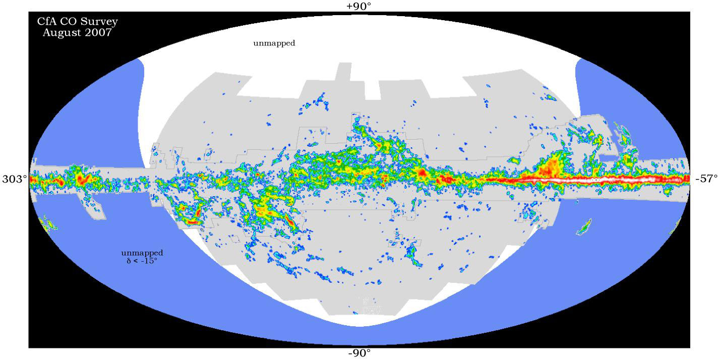
Radio astronomy has resulted in the detection of over a hundred interstellar species, including radicals and ions, and organic (i.e. carbon-based) compounds, such as alcohols, acids, aldehydes, and ketones. One of the most abundant interstellar molecules, and among the easiest to detect with radio waves (due to its strong electric dipole moment), is CO (carbon monoxide). In fact, CO is such a common interstellar molecule that it is used to map out molecular regions.[61] The radio observation of perhaps greatest human interest is the claim of interstellar glycine,[62] the simplest amino acid, but with considerable accompanying controversy.[63] One of the reasons why this detection [is] controversial is that although radio (and some other methods like rotational spectroscopy) are good for the identification of simple species with large dipole moments, they are less sensitive to more complex molecules, even something relatively small like amino acids.
"Interstellar gas in our Galaxy [shown at right] emits spectral lines as well as continuum noise. Neutral hydrogen (HI) gas is ubiquitous in the disk. The brightness of the λ ~ 21 cm hyperfine line at ~ 1420.4 MHz is proportional to the column density of HI along the line of sight and is nearly independent of the gas temperature. It is not affected by dust absorption, so we can see the HI throughout our Galaxy and nearby external galaxies."[6]
"Red indicates directions of high HI column density, while blue and black show areas with little hydrogen. The figure is centered on the Galactic center and Galactic longitude increases to the left. Some of the hydrogen loops outline old supernova remnants."[6]
Molecular clouds
G0.253+0.016 was probed "with another network of telescopes, the Combined Array for Research in Millimeter-wave Astronomy [CARMA] in California."[64]
"G0.253+0.016, which is about 30 light-years long, defies the conventional wisdom that dense gas glouds should produce lots of stars. ... The cloud is 25 times more dense than the famous Orion Nebula, which is birthing stars at a furious rate. But only a few stars are being born in G0.253+0.016, and they're pretty much all runts."[64]
"It's a very dense cloud and it doesn't form any massive stars, which is very weird"[64].
"CARMA data showed that gas within G0.253+0.016 is zipping around 10 times faster than gas in similar clouds. G0.253+0.016 is on the verge of flying apart, with its gas churning too violently to coalesce into stars. Further, the ... cloud is full of silicon monoxide, a compound typically produced when fast-moving gas smashes into dust particles. The abnormally large amounts of silicon monoxide suggest that G0.253+0.016 may actually consist of two colliding clouds, whose impact is generating powerful shockwaves."[64]
When surveyed at 1.1 mm as part of the Bolocam Galactic Plane Survey, "[t]he only currently known starless [massive proto-cluster] MPC is G0.253+0.016, which lies within the dense central molecular zone and is subject to greater environmental stresses than similar objects in the Galactic plane (Longmore et al. 2012)."[65]
Milky Way
"The cosmic static discovered by Karl Jansky is dominated by diffuse emission orginating in and near the disk of our Galaxy. The distribution of 408 MHz continuum emission shown [at right] in Galactic coordinates is expected since we are located in the disk of a galaxy similar to the edge-on galaxy NGC 4565".[6]
"This all-sky 408 MHz continuum image [at right] is shown in Galactic coordinates, with the galactic center in the middle and the galactic disk extending horizontally from it."[6]
Galaxies
"Over the past 30 years, radioastronomy has revealed a rich variety of molecular species in the interstellar medium of our galaxy and even others."[66]
These regions are non-luminous, save for emission of the 21-cm (1,420 MHz) region spectral line. ... Mapping H I emissions with a radio telescope is a technique used for determining the structure of spiral galaxies.
"In 1974, radio sources were divided into two classes Fanaroff and Riley Class I (FRI), and Class II (FRII).[67]
The distinction was originally made based on the morphology of the large-scale radio emission (the type was determined by the distance between the brightest points in the radio emission): FRI sources were brightest towards the centre, while FRII sources were brightest at the edges.
There is a reasonably sharp divide in luminosity between the two classes: FRIs were low-luminosity, FRIIs were high luminosity.[67]
The morphology turns out to reflect the method of energy transport in the radio source. FRI objects typically have bright jets in the centre, while FRIIs have faint jets but bright hotspots at the ends of the lobes. FRIIs appear to be able to transport energy efficiently to the ends of the lobes, while FRI beams are inefficient in the sense that they radiate a significant amount of their energy away as they travel.
The FRI/FRII division depends on host-galaxy environment in the sense that the FRI/FRII transition appears at higher luminosities in more massive galaxies.[68] FRI jets are known to be decelerating in the regions in which their radio emission is brightest,[69]
The hotspots that are usually seen in FRII sources are interpreted as being the visible manifestations of shocks formed when the fast, and therefore supersonic, jet (the speed of sound cannot exceed c/√3) abruptly terminates at the end of the source, and their spectral energy distributions are consistent with this picture.[70]
Recent history
The recent history period dates from around 1,000 b2k to present.
The Kulmhotel Gornergrat, atop Gorgergrat, which is both mountain and ski slope, is also home to two observatories. The Kölner Observatorium für SubMillimeter Astronomie (KOSMA) [at right] is a 3-m radio telescope located at 3,135 m on Gornergrat near Zermatt (Switzerland) in the southern tower (nearest to the camera).
"Because of the good climatic conditions at the altitude of 3135 m (10285 ft), astronomical observatories have been located in both towers of the “Kulmhotel” at Gornergrat since 1967. In 1985, the KOSMA telescope was installed in the southern tower by the Universität zu Köln and, in the course of 1995, replaced by a new dish and mount."[71]
"The KOSMA telescope with its receivers and spectrometers was dedicated to observe interstellar and atmospheric molecular lines in the millimeter and submillimeter wavelength range. After 25 years of a successful era came to an end (June 2nd, 2010). The 3m KOSMA Radio Telescope left the Gornergrat and joined his long journey to Yangbajing / Lhasa / Tibet."[71]
"Chinese and German scientists are establishing an astronomical observatory in a Tibetan county 4,300 meters above sea level."[72]
"Tibet is an ideal location because the water deficit in its air ensures superb atmospheric transparency and creates a comparatively stable environment for research in the areas of astrophysics, high-energy and atmospheric physics."[73]
"The observatory would house a KOSMA 3-meter sub-millimeter-wave telescope, the first of its kind to be used in general astronomical observation in China."[73]
Sciences
A "catalogue of 800 compact radio sources in the declination range 35° ≤ δ ≤ 75° whose positions have been measured to an rms accuracy of ~ 12 milliarcsec with the VLA [where the] observations were carried out in three sessions between 1990 February 19 and 23."[74] is available and this primary source mentions earlier catalogues.
Balloons
The E and B Experiment (EBEX) will measure the cosmic microwave background radiation of a part of the sky during two sub-orbital (high altitude) balloon flights. It is an experiment to make large, high-fidelity images of the CMB polarization anisotropies. By using a telescope which flies at over 42,000 metres high, it is possible to reduce the atmospheric absorption of microwaves to a minimum. This allows massive cost reduction compared to a satellite probe, though only a small part of the sky can be scanned and for shorter duration than a typical satellite mission such as WMAP.
EBEX was launched on 29 December, 2012, near McMurdo Station in Antarctica.[75][76]
"EBEX is meant to hone in on one specific feature of the CMB light that's been predicted, but never seen — a signature called B-type polarization, thought to have been produced by the gravity waves created by the universe's extremely rapid infant expansion, which happened even before the CMB light was released."[77]
Satellites
The image on the right shows the fairling of the Delta 1913 (D-95) being installed around Explorer 49 (RAE-B).
On the left, a Delta 1000 series rocket, serial number 95, sits on its pad at Cape Canaveral ready to launch the Explorer 49 spacecraft into a lunar orbit.
Explorer 49
Several satellites have served as observatories for radio waves and specifically for microwaves.
Explorer 49 is a 328 kilogram satellite launched on June 10, 1973 for longwave radio astronomy research. It had four 230-meter long X-shaped antenna elements, which made it one of the largest spacecraft ever built. Explorer 49 was placed into lunar orbit to provide radio astronomical measurements of the planets, the sun, and the galaxy over the frequency range of 25 kHz to 13.1 MHz.
Radio observatories
The "Arecibo Observatory in Puerto Rico [is] the world's largest, and most sensitive, single-dish radio telescope."[78]
"The 1,000-foot-diameter (305 meters) Arecibo telescope [... provides] access to state-of-the-art observing for scientists in radio astronomy, solar system radar and atmospheric studies, and the observatory has the unique capability for solar system and ionosphere (the atmosphere's ionized upper layers) radar remote sensing."[78]
"It contains the largest curved focusing dish on Earth, giving Arecibo the largest electromagnetic-wave-gathering capacity.[79] The dish surface is made of 38,778 perforated aluminum panels, each measuring about 3 by 6 feet (1 by 2 m), supported by a mesh of steel cables.
The telescope has three radar transmitters, with effective isotropic radiated powers of 20 TW at 2380 MHz, 2.5 TW (pulse peak) at 430 MHz, and 300 MW at 47 MHz. The telescope is a spherical reflector, not a parabolic reflector. To aim the telescope, the receiver is moved to intercept signals reflected from different directions by the spherical dish surface. A parabolic mirror would induce a varying astigmatism when the receiver is in different positions off the focal point, but the error of a spherical mirror is the same in every direction.
The receiver is located on a 900-ton platform which is suspended 150 m (500 ft) in the air above the dish by 18 cables running from three reinforced concrete towers, one of which is 110 m (365 ft) high and the other two of which are 80 m (265 ft) high (the tops of the three towers are at the same elevation). The platform has a 93-meter-long rotating bow-shaped track called the azimuth arm on which receiving antennas, secondary and tertiary reflectors are mounted. This allows the telescope to observe any region of the sky within a forty-degree cone of visibility about the local zenith (between −1 and 38 degrees of declination). Puerto Rico's location near the equator allows Arecibo to view all of the planets in the Solar System, though the round trip light time to objects beyond Saturn is longer than the time the telescope can track it, preventing radar observations of more distant objects.
Goldstone Deep Space Communication Complex
Shown at right are the three "34m (110 ft.) diameter Beam Waveguide antennas located at the Goldstone Deep Space Communications Complex, situated in the Mojave Desert in California. This is one of three complexes which comprise NASA's Deep Space Network (DSN). The DSN provides radio communications for all of NASA's interplanetary spacecraft and is also utilized for radio astronomy and radar observations of the solar system and the universe."[80]
Radio telescopes
A radio telescope is a form of direction radio antenna, as used in tracking and collecting data from satellites and space probes that operates in the radio frequency portion of the electromagnetic spectrum. Radio telescopes are typically large parabolic ("dish") antennas used singly or in an array. Radio observatories are preferentially located far from major centers of population to avoid electromagnetic interference (EMI) from radio, TV, radar, and other EMI emitting devices.
"The Rapid Prototype Array [RPA] observed the Navstar/GPS satellite #35 on 10 April 2001."[81]
"Data were obtained at 17:58 UT 10 April 2001. The expected location of the satellite at the RPA site was azimuth 68.7 deg, elevation 57.8 deg. Six antennas were used. Antenna one was pointed to put the satellite in the main beam. Antennas two through six were pointed to put the satellite at azimuth 68 and elevation 66."[81]
"The data-taking was triggered with a rapidly rising edge to the A/D converter. The data are synchronized to approximately 100 nsec. No compensation was made for geometric or instrumental delays."[81]
"Data were obtained in two polarizations for each antenna with 30 Msamples/sec sampling. Sample bytes were 8-bits in length. Zero voltage corresponds to approximately 127.5 counts."[81]
"Local oscillators were set so that 1575.42 MHz was mixed to 7.5 MHz before sampling. A 10 MHz IF passband filter sets the usable range of the band from 1570 to 1580 MHz, roughly."[81]
Radio interferometry
An astronomical interferometer is an array of telescopes or mirror segments acting together to probe structures with higher resolution by means of interferometry. The benefit of the interferometer is that the angular resolution of the instrument is nearly that of a telescope with the same aperture as a single large instrument encompassing all of the individual photon-collecting sub-components. The drawback is that it does not collect as many photons as a large instrument of that size. Thus it is mainly useful for fine resolution of the more luminous astronomer]]s.
Very Long Baseline Interferometry uses a technique related to the closure phase to combine telescopes separated by thousands of kilometers to form a radio interferometer with the resolution which would be given by a single dish which was thousands of kilometers in diameter. Astronomical interferometers can produce higher resolution astronomical images than any other type of telescope. At radio wavelengths image resolutions of a few micro-arcseconds have been obtained.
Hypotheses
- Radio rays can be accelerated above light speed using other photons.
Acknowledgements
The content on this page was first contributed by: Henry A. Hoff.
Initial content for this page in some instances came from Wikiversity.
See also
References
- ↑ 1.0 1.1 1.2 1.3 Cox, A. N., ed. (2000). Allen's Astrophysical Quantities. New York: Springer-Verlag. p. 124. ISBN 0-387-98746-0.
- ↑ F. H. Shu (1982). The Physical Universe. Mill Valley, California: University Science Books. ISBN 0-935702-05-9.
- ↑ Institute for Astronomy – University of Hawaii (January 2009). Mauna Kea Comprehensive Management Plan: UH Management Areas. Hawai`i State Department of Land and Natural Resources. Retrieved August 19, 2010.
- ↑ National Natural Landmark. National Park Service. Retrieved 12 December 2012.
- ↑ Mauna Kea Telescopes. Institute for Astronomy – University of Hawaii. Retrieved August 29, 2010.
- ↑ 6.00 6.01 6.02 6.03 6.04 6.05 6.06 6.07 6.08 6.09 6.10 6.11 S.G. Djorgovski; et al. A Tour of the Radio Universe. National Radio Astronomy Observatory. Retrieved 2014-03-16.
- ↑ TheDaveRoss (2 September 2006). "radio astronomy". San Francisco, California: Wikimedia Foundation, Inc. Retrieved 23 July 2019.
- ↑ http://tesla.hamradioindia.com/teslamarc.html
- ↑ http://www.teslasociety.com/father_of_radio.htm
- ↑ Christopher Bird and Oliver Nichelson. Nikola Tesla: Great Scientist, Forgotten Genius (PDF). Comcast. Retrieved 2013-06-19.
- ↑ J.S. Hey (1973). The Evolution of Radio Astronomy. Histories of Science Series. 1. Paul Elek (Scientific Books).
- ↑ Nola Taylor Redd (September 4, 2012). Meteoroids Change Atmospheres of Earth, Mars, Venus. Space.com. Retrieved 2012-09-05.
- ↑ Pozar, David M. (1993). Microwave Engineering Addison-Wesley Publishing Company. ISBN 0-201-50418-9.
- ↑ http://www.google.com/search?hl=en&defl=en&ei=e6CMSsWUI5OHmQee2si1DQ&sa=X&oi=glossary_definition&ct=title
- ↑ GRACE Launch Press Kit (PDF). NASA/JPL.
- ↑ 16.0 16.1 16.2 Morrison P (1967). "Extrasolar X-ray Sources". Ann Rev Astron Astrophys. 5 (1): 325. Bibcode:1967ARA&A...5..325M. doi:10.1146/annurev.aa.05.090167.001545.
- ↑ Iosif Shklovskii (1953). "On the Nature of the Crab Nebula's Optical Emission". Doklady Akademii Nauk SSSR. 90: 983. Bibcode:1957SvA.....1..690S.
- ↑ B. J. Burn (1973). "A synchrotron model for the continuum spectrum of the Crab Nebula". Monthly Notices of the Royal Astronomical Society. 165: 421. Bibcode:1973MNRAS.165..421B.
- ↑ White, M. (1999). Anisotropies in the CMB. UCLA. arXiv:astro-ph/9903232. Bibcode:1999dpf..conf.....W. Retrieved 2008-12-18.
- ↑ Penzias, A.A.; Wilson, R.W. (1965). "A Measurement of Excess Antenna Temperature at 4080 Mc/s". Astrophysical Journal. 142: 419–421. Bibcode:1965ApJ...142..419P. doi:10.1086/148307.
- ↑ Fixsen, D. J. (2009). "The Temperature of the Cosmic Microwave Background". The Astrophysical Journal. 707 (2): 916–920. Bibcode:2009ApJ...707..916F. doi:10.1088/0004-637X/707/2/916. Unknown parameter
|month=ignored (help) - ↑ A. J. Barger, L. L. Cowie, D. B. Sanders (1999). "Resolving the submillimeter background: the 850 micron galaxy counts". The Astrophysical Journal. 518 (1): L5–8. doi:10.1086/312054. Retrieved 2013-10-22. Unknown parameter
|month=ignored (help) - ↑ 23.0 23.1 G. Trottet, Säm Krucker, T. Lüthi, and A. Magun (2008). "Radio Submillimeter and γ-Ray Observations of the 2003 October 28 Solar Flare". The Astrophysical Journal. 678 (1): 509. doi:10.1086/528787. Retrieved 2013-10-22. Unknown parameter
|month=ignored (help) - ↑ 24.0 24.1 24.2 24.3 24.4 24.5 I.A. Smith, R.P.J. Tilanus, J. van Paradijs, T.J. Galama, P.J. Groot, P. Vreeswijk, C. Kouveliotou, R.A.M. Wijers, and N. Tanvir (1999). "SCUBA sub-millimeter observations of gamma-ray bursters I. GRB 970508, 971214, 980326, 980329, 980519, 980703, 981220, 981226". Astronomy and Astrophysics. 347 (07): 92–8. Bibcode:1999A&A...347...92S. Retrieved 2013-10-22. Unknown parameter
|month=ignored (help) - ↑ Joint Astronomy Centre, University of British Columbia and NASA/HST (STScI) (December 6, 2011). The Whirlpool Galaxy. Hawaii, USA: Joint Astronomy Centre. Retrieved 2014-03-13.
- ↑ 26.0 26.1 Abhyankar, K.D. (1977). "A Survey of the Solar Atmospheric Models". Bull. Astr. Soc. India. 5: 40–44. Bibcode:1977BASI....5...40A.
- ↑ 27.0 27.1 Brian Dunbar (November 29, 2012). MESSENGER Finds New Evidence for Water Ice at Mercury's Poles. Retrieved 2013-10-24.
- ↑ 28.0 28.1 David Lawrence (November 29, 2012). MESSENGER Finds New Evidence for Water Ice at Mercury's Poles. Washington, DC USA: NASA. Retrieved 2013-10-24.
- ↑ 29.0 29.1 Gregory Neumann (November 29, 2012). MESSENGER Finds New Evidence for Water Ice at Mercury's Poles. Washington, DC USA: NASA. Retrieved 2013-10-24.
- ↑ David Paige (November 29, 2012). MESSENGER Finds New Evidence for Water Ice at Mercury's Poles. Washington, DC USA: NASA. Retrieved 2013-10-24.
- ↑ Steven J. Ostro (1993). "Planetary radar astronomy". Reviews of Modern Physics. 65 (4): 1235–79. doi:10.1103/RevModPhys.65.1235. Retrieved 2012-02-09. Unknown parameter
|month=ignored (help) - ↑ J. Mofensen (1946). "Radar Echoes from the Moon". Nature, Electronics. 157, 19 (3379): 129, 92–8. Bibcode:1946Natur.157R.129.. doi:10.1038/157129b0. Unknown parameter
|month=ignored (help) - ↑ Z. Bay, Reflection of microwaves from the moon," Hung. Acta Phys., vol. 1, pp. 1-22; April, 1946.
- ↑ 34.0 34.1 Tony Greicius (December 6, 2012). GRAIL's Gravity Map of the Moon. NASA/JPL-Caltech/MIT/GSFC. Retrieved 2012-12-15.
- ↑ 35.0 35.1 35.2 35.3 35.4 35.5 PR Newswire (December 5, 2012). NASA Twin Spacecraft Create Most Accurate Gravity Map Of Moon. Retrieved 2012-12-15.
- ↑ 36.0 36.1 36.2 36.3 36.4 P. Spudis (November 6, 2006). Ice on the Moon. The Space Review. Retrieved 12 April 2007.
- ↑ B. Gardini (2011). "ESA strategy for human exploration and the Lunar Lander Mission". Memorie della Societa Astronomica Italiana. 82: 422–29. Bibcode:2011MmSAI..82..422G. Retrieved 5 May 2019.
- ↑ Jokipii (1973), pp. 11–12.
- ↑ Alurkar (1997), p. 11.
- ↑ BatteryIncluded (June 14, 2013). File:PIA13164 North Polar Cap Cross Section, Annotated Version.jpg. San Francisco, California: Wikimedia Foundation, Inc. Retrieved 2013-10-24.
- ↑ 41.0 41.1 41.2 Thomas Thompson (September 2, 2013). Radar Ionogram with Oblique Ionospheric Echo. Pasadena, California USA: NASA. Retrieved 2013-10-24.
- ↑ 42.0 42.1 42.2 42.3 42.4 42.5 42.6 Sue Lavoie (December 13, 2006). PIA09076: Interpreting Radar View near Mars' South Pole, Orbit 1334. Pasadena, California USA: NASA. Retrieved 2013-10-24.
- ↑ 43.0 43.1 43.2 Ian O'Neill (June 22, 2012). Asteroid 2012 LZ1 Just Got Supersized. Discovery Communications, LLC. Retrieved 2013-10-24.
- ↑ Ellen Howell (June 22, 2012). Asteroid 2012 LZ1 Just Got Supersized. Discovery Communications, LLC. Retrieved 2013-10-24.
- ↑ Mike Nolan (June 22, 2012). Asteroid 2012 LZ1 Just Got Supersized. Discovery Communications, LLC. Retrieved 2013-10-24.
- ↑ 46.0 46.1 Don Savage and Jane Platt (November 27, 1996). Images of Asteroid 4179 Toutatis. Washington, DC USA: NASA. Retrieved 2013-10-24.
- ↑ 47.0 47.1 Eric De Jong (November 27, 1996). Images of Asteroid 4179 Toutatis. Washington, DC USA: NASA. Retrieved 2013-10-24.
- ↑ 48.0 48.1 Scott Hudson (November 27, 1996). Images of Asteroid 4179 Toutatis. Washington, DC USA: NASA. Retrieved 2013-10-24.
- ↑ 49.0 49.1 49.2 Steven Ostro (November 27, 1996). Images of Asteroid 4179 Toutatis. Washington, DC USA: NASA. Retrieved 2013-10-24.
- ↑ 50.0 50.1 Linda T. Elkins-Tanton (2006). Jupiter and Saturn. New York: Chelsea House. ISBN 0-8160-5196-8.
- ↑ Weintraub, Rachel A. (September 26, 2005). How One Night in a Field Changed Astronomy. NASA. Retrieved 2007-02-18.
- ↑ Garcia, Leonard N. The Jovian Decametric Radio Emission. NASA. Retrieved 2007-02-18.
- ↑ Klein, M. J.; Gulkis, S.; Bolton, S. J. (1996). Jupiter's Synchrotron Radiation: Observed Variations Before, During and After the Impacts of Comet SL9. NASA. Retrieved 2007-02-18.
- ↑ 54.0 54.1 Gordon H. Pettengill & Irwin I. Shapiro (1965). "Radar Astronomy". Annual Review of Astronomy and Astrophysics. 3: 377–410. Bibcode:1965ARA&A...3..377P. Retrieved 2012-12-25.
- ↑ Irwin I. Shapiro (1968). "Planetary radar astronomy". Spectrum, IEEE. 5 (3): 70–9. doi:10.1109/MSPEC.1968.5214821. Retrieved 2012-12-25. Unknown parameter
|month=ignored (help) - ↑ R. B. Dyce and G. H. Pettengill, and A. D. Sanchez (1967). "Radar Observations of Mars and Jupiter at 70 cm" (PDF). The Astronomical Journal. 72 (4): 771–7. Bibcode:1967AJ.....72..771D. doi:10.1086/110307. Retrieved 2012-12-25. Unknown parameter
|month=ignored (help) - ↑ 57.0 57.1 57.2 57.3 Enrico Piazza (May 23, 2005). Waves and Small Particles in Ring A. Pasadena, California USA: NASA/JPL. Retrieved 2013-03-27.
- ↑ 58.0 58.1 58.2 58.3 58.4 Sue Lavoie (October 11, 2007). PIA10008: Titan's North Polar Region. Pasadena, California USA: NASA/JPL. Retrieved 2013-06-13.
- ↑ 59.0 59.1 59.2 59.3 Enrico Piazza (January 3, 2007). Liquid Lakes on Titan. Pasadena, California USA: NASA/JPL. Retrieved 2013-06-13.
- ↑ Fernando Simões (June 1, 2007). Titan’s mysterious radio wave. ESA. Retrieved 2012-08-30.
- ↑ http://www.cfa.harvard.edu/mmw/CO_survey_aitoff.jpg.
- ↑ Kuan YJ, Charnley SB, Huang HC; et al. (2003). "Interstellar glycine". The Astrophysical Journal. 593 (2): 848–867. Bibcode:2003ApJ...593..848K. doi:10.1086/375637.
- ↑ Snyder LE, Lovas FJ, Hollis JM; et al. (2005). "A rigorous attempt to verify interstellar glycine". The Astrophysical Journal. 619 (2): 914–30. arXiv:astro-ph/0410335. Bibcode:2005ApJ...619..914S. doi:10.1086/426677.
- ↑ 64.0 64.1 64.2 64.3 SPACE.com Staff (January 14, 2013). Baffling Star Birth Mystery Finally Solved. Yahoo! Inc. Retrieved 2013-01-15.
- ↑ A. Ginsburg, E. Bressert, J. Bally, C. Battersby (2012). "There are No Starless Massive Proto-Clusters in the First Quadrant of the Galaxy" (PDF). The Astrophysical Journal Letters. 758 (2): L29–33. arXiv:1208.4097. Bibcode:2012ApJ...758L..29G. doi:10.1088/2041-8205/758/2/L29. Retrieved 2013-01-15. Unknown parameter
|month=ignored (help) - ↑ Dudley Herschbach (1999). "Chemical physics: Molecular clouds, clusters, and corrals". Reviews of Modern Physics. 71 (2): S411–S418. doi:10.1103/RevModPhys.71.S411. Retrieved 2011-12-17. Unknown parameter
|month=ignored (help); Unknown parameter|pdf=ignored (help) - ↑ 67.0 67.1 Fanaroff, Bernard L., Riley Julia M.; Riley (1974). "The morphology of extragalactic radio sources of high and low luminosity". Monthly Notices of the Royal Astronomical Society. 167: 31P–36P. Bibcode:1974MNRAS.167P..31F. Unknown parameter
|month=ignored (help) - ↑ Owen FN, Ledlow MJ (1994). "The FRI/II Break and the Bivariate Luminosity Function in Abell Clusters of Galaxies". In G.V. Bicknell, M.A. Dopita, and P.J. Quinn, (Eds.). The First Stromlo Symposium: The Physics of Active Galaxies. ASP Conference Series,. 54. Astronomical Society of the Pacific Conference Series. p. 319. ISBN 0-937707-73-2.
- ↑ Laing RA, Bridle AH (2002). "Relativistic models and the jet velocity field in the radio galaxy 3C31". Monthly Notices of the Royal Astronomical Society. 336 (1): 328–57. arXiv:astro-ph/0206215. Bibcode:2002MNRAS.336..328L. doi:10.1046/j.1365-8711.2002.05756.x.
- ↑ Meisenheimer K, Röser H-J, Hiltner PR, Yates MG, Longair MS, Chini R, Perley RA; Roser; Hiltner; Yates; Longair; Chini; Perley (1989). "The synchrotron spectra of radio hotspots". Astronomy and Astrophysics. 219: 63–86. Bibcode:1989A&A...219...63M.
- ↑ 71.0 71.1 Fachgruppe Physik (June 2, 2010). KOSMA. Köln, Deutschland: Universität zu Köln. Retrieved 2014-03-12.
- ↑ Wang Junjie (October 2010). China, Germany Build Astronomical Observatory in Tibet. People's Republic of China: Chinese Academy of Sciences. Retrieved 2014-03-12.
- ↑ 73.0 73.1 Yan Jun (October 2010). China, Germany Build Astronomical Observatory in Tibet. People's Republic of China: Chinese Academy of Sciences. Retrieved 2014-03-12.
- ↑ Alok R. Patnaik, Ian W. A. Browne, Peter N. Wilkinson and Joan M. Wrobel (1992). "Interferometer phase calibration sources. I - The region 35-75 deg". Monthly Notices of the Royal Astronomical Society. 254 (02): 655–76. Bibcode:1992MNRAS.254..655P. Retrieved 2014-02-28. Unknown parameter
|month=ignored (help) - ↑ Blog post from a member of the EBEX science team describing the launch.
- ↑ YouTube video of the EBEX launch.
- ↑ Clara Moskowitz (February 4, 2013). Balloon-Borne Telescope Seeks Out Elusive Big Bang Signal. Yahoo! News. Retrieved 2013-02-05.
- ↑ 78.0 78.1 David Brand (21 January 2003). Astrophysicist Robert Brown, leader in telescope development, named to head NAIC and its main facility, Arecibo Observatory. Cornell University. Retrieved 2008-09-02.
- ↑ Frederic Castel (8 May 2000). Arecibo: Celestial Eavesdropper. Space.com. Retrieved 2008-09-02.
- ↑ Michael Hahn (January 1, 1990). Goldstone Deep Space Communication Complex. Washington, DC USA: NASA HQ. Retrieved 2013-10-24.
- ↑ 81.0 81.1 81.2 81.3 81.4 Geoffrey C. Bower (2 August 2001). Application of Wiener and Adaptive Filters to GPS and Glonass Data from the Rapid Prototyping Array (PDF). Lafayette, California USA: SETI.org. Retrieved 2016-09-23.
Further reading
- Cox, A. N., ed. (2000). Allen's Astrophysical Quantities. New York: Springer-Verlag. p. 124. ISBN 0-387-98746-0.
- F. H. Shu (1982). The Physical Universe. Mill Valley, California: University Science Books. ISBN 0-935702-05-9.
External links
- Bing Advanced search
- Google Books
- Google scholar Advanced Scholar Search
- The History of Radio Astronomy
- International Astronomical Union
- JSTOR
- Lycos search
- NASA/IPAC Extragalactic Database - NED
- nrao.edu National Radio Astronomy Observatory
- NASA's National Space Science Data Center
- NCBI All Databases Search
- Office of Scientific & Technical Information
- PubChem Public Chemical Database
- Questia - The Online Library of Books and Journals
- SAGE journals online
- The SAO/NASA Astrophysics Data System
- Scirus for scientific information only advanced search
- SDSS Quick Look tool: SkyServer
- SIMBAD Astronomical Database
- Spacecraft Query at NASA
- SpringerLink
- Taylor & Francis Online
- Universal coordinate converter
- Wiley Online Library Advanced Search
- Yahoo Advanced Web Search
{{Charge ontology}}{{Chemistry resources}}{{Geology resources}}{{Principles of radiation astronomy}}Editor-In-Chief: Henry A Hoff